Student’s t: location-scale
Motivation
Often when we examine financial data, we find that logarithmic returns exhibit fatter tails than the normal distribution. Hence, we need a distribution with more probability mass in the tails, and – coming from traditional financial mathematics with normally distributed log-returns – the natural first choice is the student’s 
However, the standard student’s
Standard student’s t-distribution
For 


## set parameter
nu <- 8

## number of samples
n <- 10000

## simulate
t <- rt(n,nu)

## analytically calculated variance
variance <- nu/(nu-2)
sprintf("True variance: %f",variance)

## get sample variance
sprintf( "Sample variance: %f",var(t))
: [1] “True variance: 1.333333” : [1] “Sample variance: 1.291841”
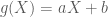
Location-scale transformation
Through application of a linear transformation, we can easily shift the center of the distribution and affect the divergence from its mean.
![\displaystyle \begin{aligned} Y&=aX + b,\quad X\sim t \\ \mathbb{E}[Y]&=b \\ \mathbb{V}(Y)&=a^{2}\mathbb{V}(X) \\ &=a^{2} \frac{\nu}{\nu-2} \end{aligned}](https://s0.wp.com/latex.php?latex=%5Cdisplaystyle+%5Cbegin%7Baligned%7D+Y%26%3DaX+%2B+b%2C%5Cquad+X%5Csim+t+%5C%5C+%5Cmathbb%7BE%7D%5BY%5D%26%3Db+%5C%5C+%5Cmathbb%7BV%7D%28Y%29%26%3Da%5E%7B2%7D%5Cmathbb%7BV%7D%28X%29+%5C%5C+%26%3Da%5E%7B2%7D+%5Cfrac%7B%5Cnu%7D%7B%5Cnu-2%7D+%5Cend%7Baligned%7D&bg=ffffff&fg=4e4e4e&s=0&c=20201002)
Note, that the standard deviation of the new random variable 

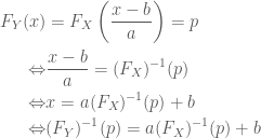
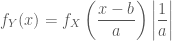
The cumulative distribution function after the transformation can easily be obtained through:

Taking this result, we can derive the inverse cdf:
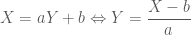
Getting the density of

with 
Calculating 

Taking the derivative:
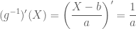
Putting the parts together, we get:
Implementation
The functions now can be implemented in R. We use the code provided by wikipedia:
dt_ls <- function(x, df, mu, a) 1/a * dt((x - mu)/a, df)
pt_ls <- function(x, df, mu, a) pt((x - mu)/a, df)
qt_ls <- function(prob, df, mu, a) qt(prob, df)*a + mu
rt_ls <- function(n, df, mu, a) rt(n,df)*a + mu
We can now try to fit the t-location-scale distribution to simulated data.
library(MASS)

## set parameters
n <- 10000
mu <- 0.4
a <- 1.2
nu <- 4

## simulate values
simVals <- rt_ls(n, nu,mu,a)
fit <- fitdistr(simVals,"t")
print(fit)
There were 12 warnings (use warnings() to see them)
       m            s            df
  0.40849216   1.20630991   4.00772609
 (0.01427656) (0.01498895) (0.16515696)
Posted on 2013/04/30, in financial econometrics, R and tagged fat_tails, location-scale, Rbloggers, Student's_t, t. Bookmark the permalink. 2 Comments.

Pingback: Model Checking: Posterior Predictive Checks – Laplace Bayes
Pingback: Model Checking: Posterior Predictive Checks – DataCATz